Here are yet more tools that the average user won’t need, but might come in handy one day.
Nested dictionaries
Nested dictionaries are a useful way of storing complex data (and in fact are more or less the basis of JSON), but can be a pain to interact with if you don’t know the structure in advance. Sciris has several functions for working with nested dictionaries. For example:
import sciris as sc# Create the structurenest = {}sc.makenested(nest, ['key1','key1.1'])sc.makenested(nest, ['key1','key1.2'])sc.makenested(nest, ['key1','key1.3'])sc.makenested(nest, ['key2','key2.1','key2.1.1'])sc.makenested(nest, ['key2','key2.2','key2.2.1'])# Set the value for each "twig"count =0for twig in sc.iternested(nest): count +=1 sc.setnested(nest, twig, count)# Convert to a JSON to view the structure more clearlysc.printjson(nest)# Get all the values from the dictvalues = []for twig in sc.iternested(nest): values.append(sc.getnested(nest, twig))print(f'{values =}')
Sciris contains two context block (i.e. “with ... as”) classes for catching what happens inside them.
sc.capture() captures all text output to a variable:
import sciris as scimport numpy as npdef verbose_func(n=200):for i inrange(n):print(f'Here are 5 random numbers: {np.random.rand(5)}')with sc.capture() as text: verbose_func()lines = text.splitlines()target ='777'for l,line inenumerate(lines):if target in line:print(f'Found target {target} on line {l}: {line}')
Found target 777 on line 63: Here are 5 random numbers: [0.52531775 0.57771242 0.35008666 0.62236895 0.60116745]
Found target 777 on line 68: Here are 5 random numbers: [0.95785514 0.91804777 0.79962423 0.87363375 0.20456325]
Found target 777 on line 86: Here are 5 random numbers: [0.79055969 0.16997771 0.14426824 0.62427766 0.822207  ]
Found target 777 on line 103: Here are 5 random numbers: [0.17776686 0.86880159 0.54908261 0.36875631 0.76937501]
Found target 777 on line 106: Here are 5 random numbers: [0.77712309 0.96541288 0.09278934 0.43521704 0.64319382]
Found target 777 on line 137: Here are 5 random numbers: [0.24340748 0.43510268 0.40107582 0.2687779  0.54790469]
Found target 777 on line 178: Here are 5 random numbers: [0.07421381 0.47778131 0.23940222 0.88028022 0.05084695]
The other function, sc.tryexcept(), is a more compact way of writing try ... except blocks, and gives detailed control of error handling:
def fickle_func(n=1):for i inrange(n): rnd = np.random.rand()if rnd <0.005:raiseValueError(f'Value {rnd:n} too small')elif rnd >0.99:raiseRuntimeError(f'Value {rnd:n} too big')sc.heading('Simple usage, exit gracefully at first exception')with sc.tryexcept(): fickle_func(n=1000)sc.heading('Store all history')tryexc =Nonefor i inrange(1000):with sc.tryexcept(history=tryexc, verbose=False) as tryexc: fickle_func()tryexc.disp()
————————————————————————————————————————————————

Simple usage, exit gracefully at first exception

————————————————————————————————————————————————


<class 'RuntimeError'> Value 0.995894 too big


—————————————————

Store all history

—————————————————


<sciris.sc_utils.tryexcept at 0x7f5180109ad0>

[<class 'sciris.sc_utils.tryexcept'>, <class 'contextlib.suppress'>, <class 'contextlib.AbstractContextManager'>, <class 'abc.ABC'>]

————————————————————————————————————————————————————————————————————————

Methods:

  disp()                  to_df()                 traceback()

————————————————————————————————————————————————————————————————————————

Properties:

  died                    exception               exceptions

————————————————————————————————————————————————————————————————————————

catchtypes: ()

      data: [[<class 'RuntimeError'>, RuntimeError('Value 0.994527 too

            big'), <tra [...]

defaultdie: False

  dietypes: ()

   message: ''

 outputstr: ''

   verbose: 0

 _abc_impl: <_abc._abc_data object at 0x7f5158cf4d80>

————————————————————————————————————————————————————————————————————————
Interpolation and optimization
Sciris includes two algorithms that complement their SciPy relatives: interpolation and optimization.
Interpolation
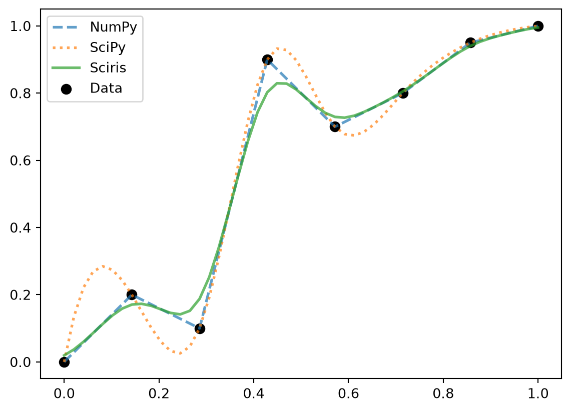
The function sc.smoothinterp() smoothly interpolates between points but does not use spline interpolation; this makes it somewhat of a balance between numpy.interp() (which only interpolates linearly) and scipy.interpolate.interp1d(..., method='cubic'), which takes considerable liberties between data points:
As you can see, sc.smoothinterp() gives a more “reasonable” approximation to the data, at the expense of not exactly passing through all the data points.
Optimization
Sciris includes a gradient descent optimization method, adaptive stochastic descent (ASD), that can outperform SciPy’s built-in optimization methods (such as simplex) for certain types of optimization problem. For example:
# Basic usageimport numpy as npimport sciris as scfrom scipy import optimize# Very simple optimization problem -- set all numbers to 0func = np.linalg.normx = [1, 2, 3]with sc.timer('scipy.optimize()'): opt_scipy = optimize.minimize(func, x)with sc.timer('sciris.asd()'): opt_sciris = sc.asd(func, x, verbose=False)print(f'Scipy result: {func(opt_scipy.x)}')print(f'Sciris result: {func(opt_sciris.x)}')
scipy.optimize(): 18.7 ms
sciris.asd(): 5.34 ms
Scipy result:  4.826351964229613e-08
Sciris result: 2.9998179386671717e-16
Compared to SciPy’s simplex algorithm, Sciris’ ASD algorithm was ≈3 times faster and found a result ≈8 orders of magnitude smaller.
Animation
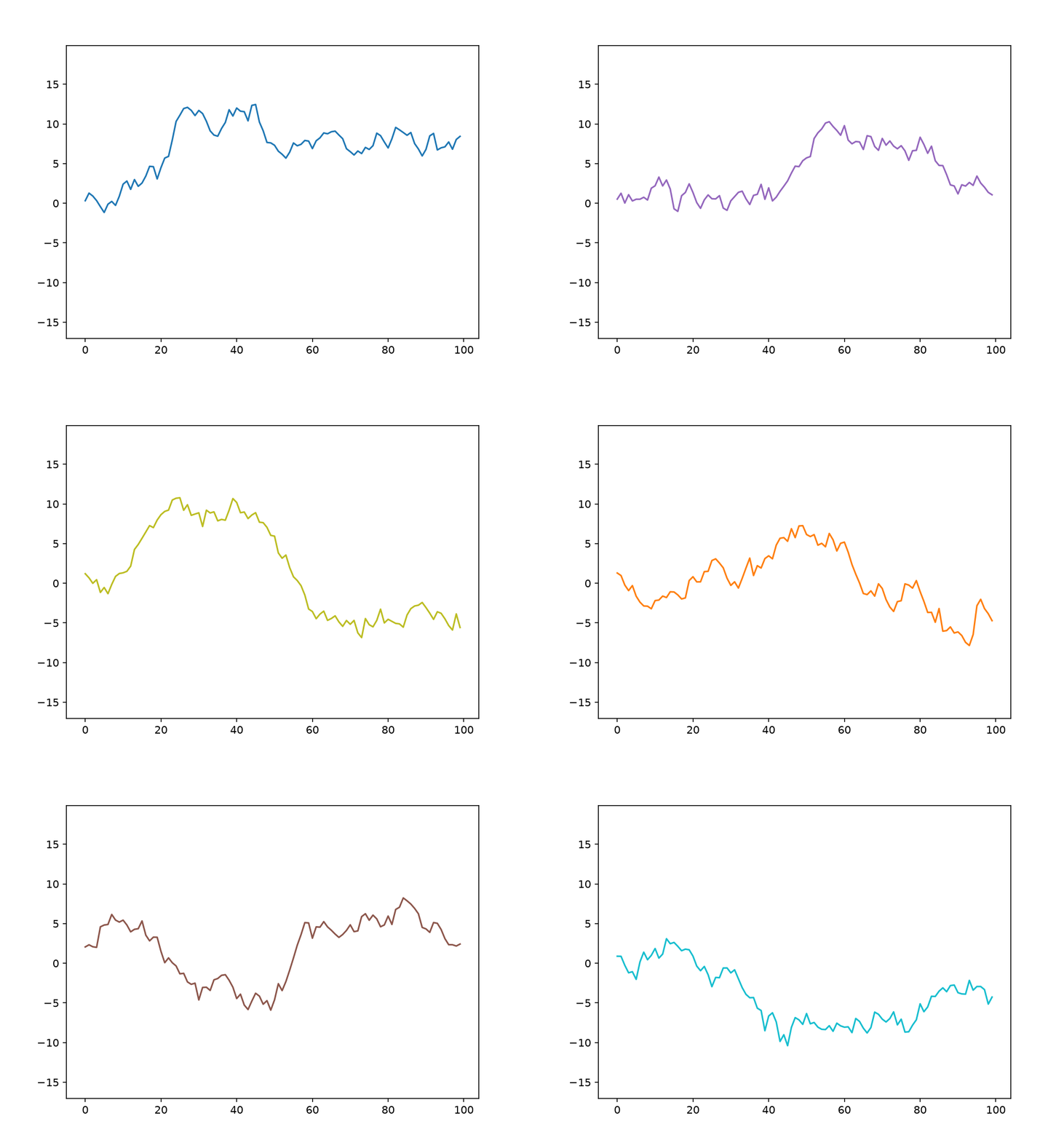
And finally, let’s end on something fun. Sciris has an sc.animation() class with lots of options, but you can also just make a quick movie from a series of plots. For example, let’s make some lines dance:
plt.figure()frames = [plt.plot(np.cumsum(np.random.randn(100))) for i inrange(20)] # Create framessc.savemovie(frames, 'dancing_lines.gif');# Save movie as a gif
MovieWriter imagemagick unavailable; using Pillow instead.
Saving 20 frames at 10 fps and 150 dpi to "dancing_lines.gif" using imagemagick...
Done; movie saved to "dancing_lines.gif"
File size: 242 KB
Elapsed time: 2.27 s
This creates the following movie, which is a rather delightful way to end:
We hope you enjoyed this series of tutorials! Remember, write to us if you want to get in touch.